We Out Here Tryin’ to Function

One of the key steps in making “improvements” on your R journey is to write code that is more clear, succinct, concise and short; for me, this usually occurs when I need to create multiple plots of variables when exploring a dataset.

I find myself usually making simple bar plots using ggplot and geom_col() to count things. Instead of copying-and-pasting the same ggplot code and altering the the column names in the code like a newbie hack, I recently learned about double curly braces “{{ }}” which allow you to dynamically pass unquoted variable names within functions.

First, we’ll use the palmerpenguins package to make some bar plots (Yeah, I am fully aware that I should’ve worked with some Spotify/Apple Music Bay Area music datasets to make this blog post even more hyphy). I examine the penguins dataset to see which columns are categorical/discrete and numerical/continuous:

library(tidyverse)
library(palmerpenguins)
theme_set(theme_minimal())

penguins %>% glimpse()

Rows: 344
Columns: 8
$ species           <fct> Adelie, Adelie, Adelie, Adelie, Adelie, Adelie, Adel…
$ island            <fct> Torgersen, Torgersen, Torgersen, Torgersen, Torgerse…
$ bill_length_mm    <dbl> 39.1, 39.5, 40.3, NA, 36.7, 39.3, 38.9, 39.2, 34.1, …
$ bill_depth_mm     <dbl> 18.7, 17.4, 18.0, NA, 19.3, 20.6, 17.8, 19.6, 18.1, …
$ flipper_length_mm <int> 181, 186, 195, NA, 193, 190, 181, 195, 193, 190, 186…
$ body_mass_g       <int> 3750, 3800, 3250, NA, 3450, 3650, 3625, 4675, 3475, …
$ sex               <fct> male, female, female, NA, female, male, female, male…
$ year              <int> 2007, 2007, 2007, 2007, 2007, 2007, 2007, 2007, 2007…

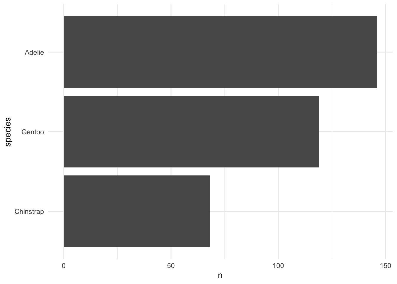
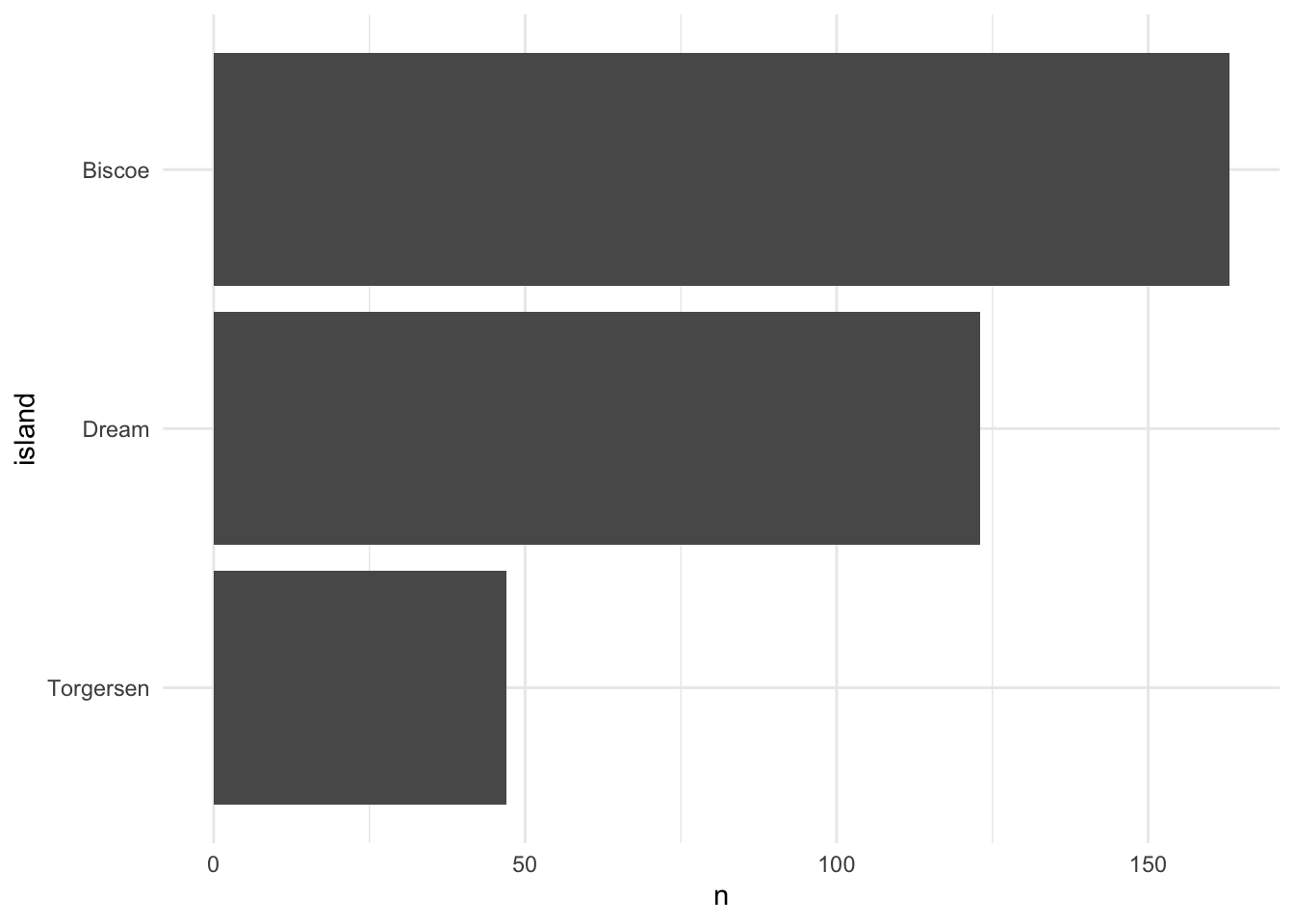
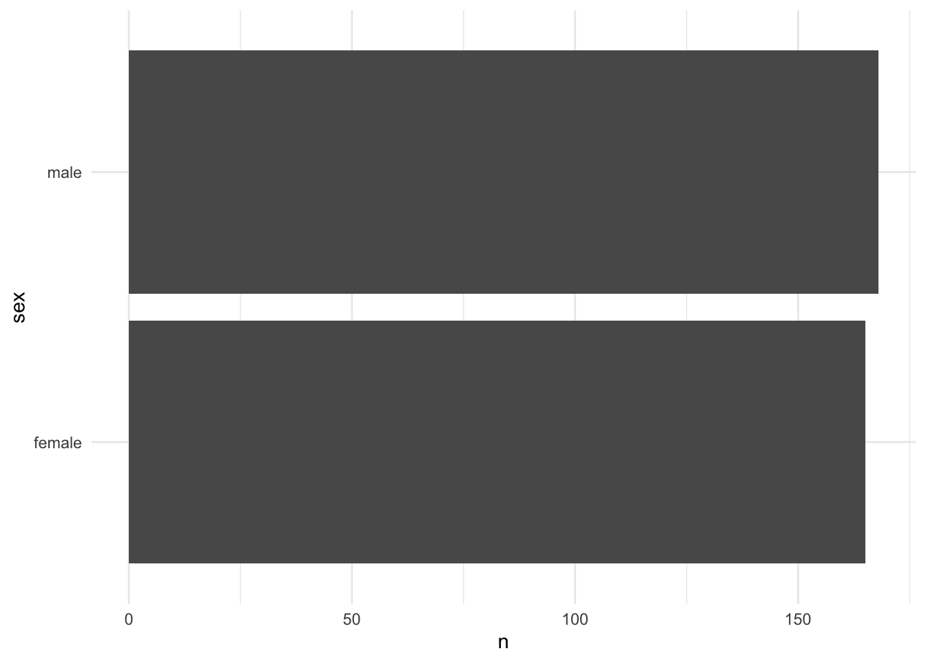
An easy first look at exploring a dataset is to simply count the number of items in a variable. I want to determine the counts across the categorical columns and make a bar plot for each. That happens to be the species, island and sex columns. Here’s the long way how to do it:

penguins %>% 
  drop_na() %>% 
  count(species, sort = TRUE) %>% 
  mutate(species = fct_reorder(species, n)) %>% 
  ggplot(aes(x = species, y = n)) + 
  geom_col() +
  coord_flip()
penguins %>% 
  drop_na() %>% 
  count(island, sort = TRUE) %>% 
  mutate(island = fct_reorder(island, n)) %>% 
  ggplot(aes(x = island, y = n)) + 
  geom_col() +
  coord_flip()
penguins %>% 
  drop_na() %>% 
  count(sex, sort = TRUE) %>% 
  mutate(sex = fct_reorder(sex, n)) %>% 
  ggplot(aes(x = sex, y = n)) + 
  geom_col() +
  coord_flip()

In the code demonstrated above, I realize that all I am just changing is the name of the columns (species, island, sex) to create the three different plots. The rule of thumb is to succint programming is to avoid duplication of code – twice is fine but thrice is too much! Here, we can attempt to create a function to shorten the number of lines written. We create a function (I named it geomcol_discrete) with the nifty use of the double curly brackets { column } to maintain a tidyverse work flow:

# function - discrete plots
geomcol_discrete <- function(tbl, column) {
  tbl %>% 
    drop_na() %>% 
    count({{ column }}, sort = TRUE) %>% 
    mutate({{ column }} := fct_reorder({{ column }}, n)) %>% 
    ggplot(aes(x = {{ column }}, y = n)) + 
    geom_col() +
    coord_flip()
}

And now we quickly plot with geomcol_discrete:

penguins %>% geomcol_discrete(species)
penguins %>% geomcol_discrete(island)
penguins %>% geomcol_discrete(sex)

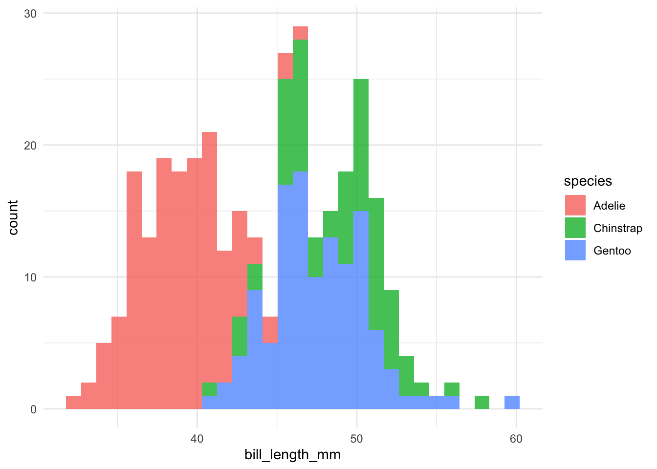
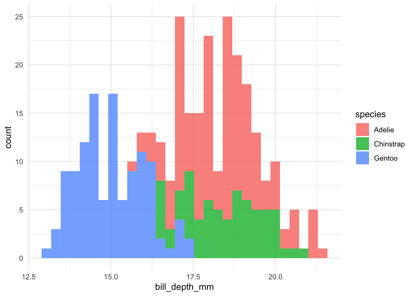
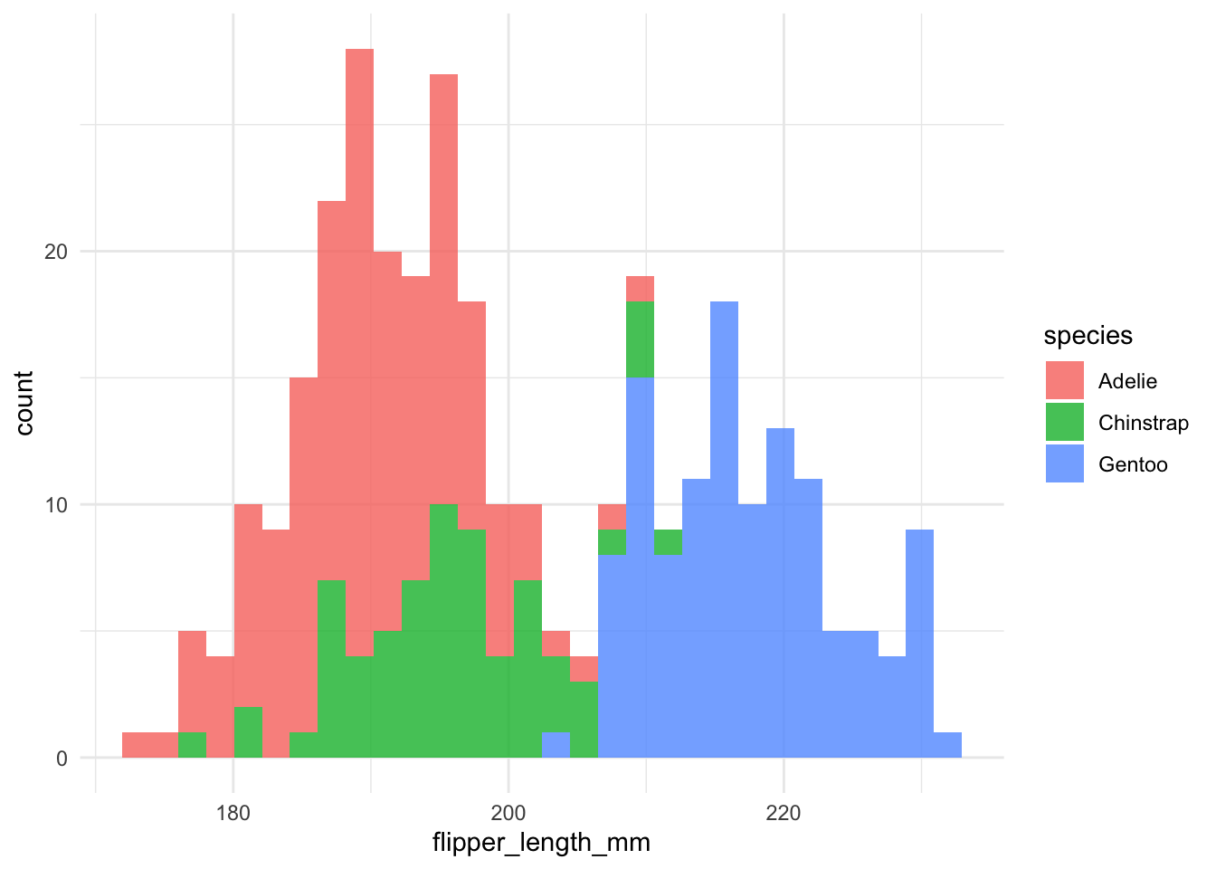
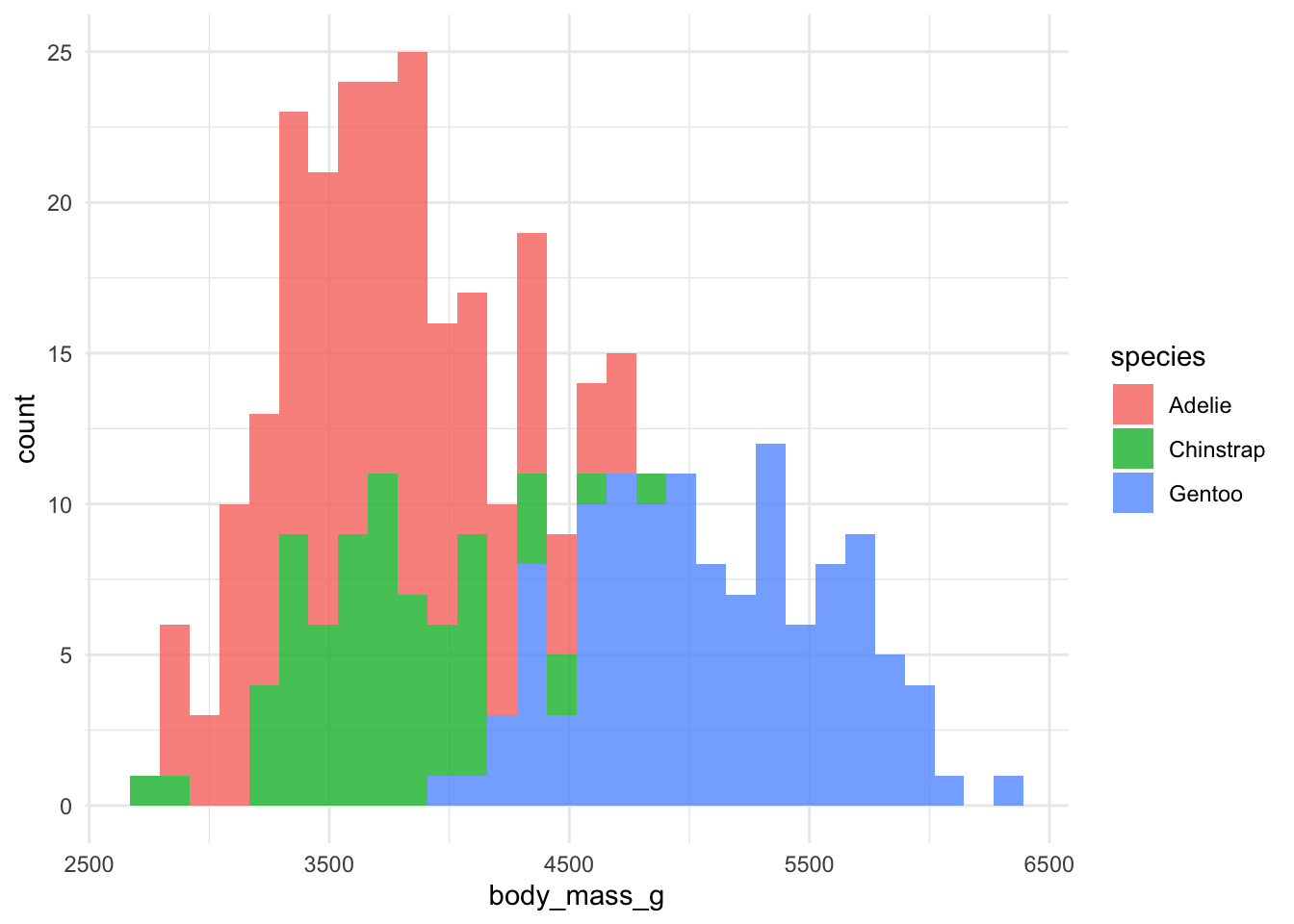
I also created a function to plot histograms for the continuous data geomhist_continuous:

# function - continuous plots
geomhist_continuous <- function(tbl, column) {
  tbl %>% 
    drop_na() %>% 
    ggplot(aes(x = {{ column }}, fill = species)) +
    geom_histogram(alpha = 0.8)
}

# now we quickly plot
penguins %>% geomhist_continuous(bill_length_mm)
penguins %>% geomhist_continuous(bill_depth_mm)
penguins %>% geomhist_continuous(flipper_length_mm)
penguins %>% geomhist_continuous(body_mass_g)

The next step further would be to create a vector of column names so that I can loop the functions. Stay tuned for a future update. As the Bay Area hip-hop lingo would dictate, We out here tryin’ to function!

bay area native H.E.R.