
As a wildlife biologist, one of the first steps in exploring spatial analyses with R is to produce a map with recorded (x, y) locations of your species of interest; for example, many researchers mark animal locations with a handheld Garmin GPS or obtain location data from GPS collars, and would like to see on a map where all the occurrences of their study animals have been recorded. I remember it took me forever just to learn this basic exercise so I thought it would be a nice blog post for students in the same position and beginning their spatial journey in becoming a SAP (Spatially Aware Professional).
For #InternationalLeopardDay, I thought it would be a fun and simple exercise to download recorded leopard (Panthera pardus) occurrence records from the GBIF database and to produce a basic leopard occurrence map.
The Global Biodiversity Information Facility (GBIF) platform provides open access to biodiversity data, where many scientists have produced species distribution models and maps to explore global ranges for various wildlife species. We’ll download leopard location data from GBIF and explore their range. Note: Like all open source databases, not all information inputted will be accurate. We’ll have to use our best judgment to identify outlier points in GBIF, which mostly are attributed to user error.
We’ll be using dismo, sf and tidyverse packages to download GBIF data and tidy our spatial data. Remember, if you’re starting to work exclusively with spatial data, sf is a package I suggest that you should spend some considerable time with.
1 Packages
2 Downloading the data
I use the gbif function to download records for leopards (Panthera pardus). I also use the option geo=FALSE to download records without numerical georeferences (records that do not come with location x,y data). nrecs is the argument to download the max number of records at a time, which is 300.
Code
# A tibble: 6 × 208
  acceptedNameUsage acceptedScientificName   acceptedTaxonKey accessRights adm1
  <chr>             <chr>                               <int> <chr>        <chr>
1 <NA>              Panthera pardus kotiya …          5219437 <NA>         Mone…
2 <NA>              Panthera pardus kotiya …          5219437 <NA>         Mone…
3 <NA>              Panthera pardus (Linnae…          5219436 <NA>         West…
4 <NA>              Panthera pardus pardus            7193915 <NA>         Nort…
5 <NA>              Panthera pardus fusca (…          5219442 <NA>         Raja…
6 <NA>              Panthera pardus pardus            7193915 <NA>         Mpum…
# ℹ 203 more variables: adm2 <chr>, associatedOccurrences <chr>,
#   associatedReferences <chr>, associatedSequences <chr>,
#   basionymAuthors <chr>, basionymYear <chr>, basisOfRecord <chr>, bed <chr>,
#   behavior <chr>, bibliographicCitation <chr>, canonicalName <chr>,
#   catalogNumber <chr>, class <chr>, classKey <int>, cloc <chr>,
#   collectionCode <chr>, collectionID <chr>, collectionKey <chr>,
#   combinationAuthors <chr>, combinationYear <chr>, continent <chr>, …
3 Tidying the data
The data tibble seems to look okay, with at least 9,882 records being downloaded. With many columns of information provided by GBIF, we are mainly interested in lon and lat (x,y data) and locality. Let’s summarize our data by determining among the downloaded records, how many have coordinates, and how many records do not have coordinates but have a textual geo-reference (locality description).
     n
1 9905
Code
# A tibble: 5 × 2
  loc                     n
  <fct>               <int>
1 NA,NA                2500
2 35.420663,31.491912   495
3 35.315413,31.492047   132
4 34.965783,32.67288     66
5 32.15,28.7666          60
Code
                                 locality n
1                            Ituri forest 1
2                             Cochinchine 2
3                           Rumathe River 1
4                 Ahl al Oughlam - Site 1 3
5                          Laristan, Fars 1
6                             Mount Elgon 1
7  Deutsch-Ostafrika (aus Familienbesitz) 1
8                                  África 1
9                              Masai Mara 1
10                              Ethiopean 2
So out of ~9,800 records downloaded, 2,500 records do not have geo-referenced coordinates and were inputted as (NA,NA) in the dataset. A lot of the records that were not geo-referenced but had a recorded locality listed were sightings of leopards from zoos, and records that wouldn’t be too particularly useful in producing a map, such as “Africa”, “on Simiyu River”, “see remarks”, etc.
4 Static Map
Now it’s time to make a simple map. We just want to use records with (lon, lat) from our pardus tibble frame. From the sf package, we want to create an sf spatial object by using the st_as_sf() function to retrieve the coordinates, and then use the st_set_crs() function for our projection of choice.
We use the geom_sf() function with ggplot2 to put all the points together on the world map. Additionally, we can use the new tm_basemap() function to spice up our tmap.
Code
# create sf obect with coordinations and projection
pardus_sf <- pardus %>%
  filter(lon != is.na(lon) | lat != is.na(lat)) %>%
  st_as_sf(coords = c("lon", "lat"), remove = FALSE) %>% # key function
  st_set_crs(4326)
# load World map from tmap package
data(World)
# combine sf objects to produce ggplot map
ggplot() +
  geom_sf(data = World) +
  geom_sf(data = pardus_sf, aes(color = "Panthera pardus"), alpha = 0.4) +
  labs(title = "Panthera pardus occurrences",
       subtitle = "Source: GBIF") +
  scale_color_manual(name = "locations",
                     values = "black") +
  theme(legend.position = "bottom")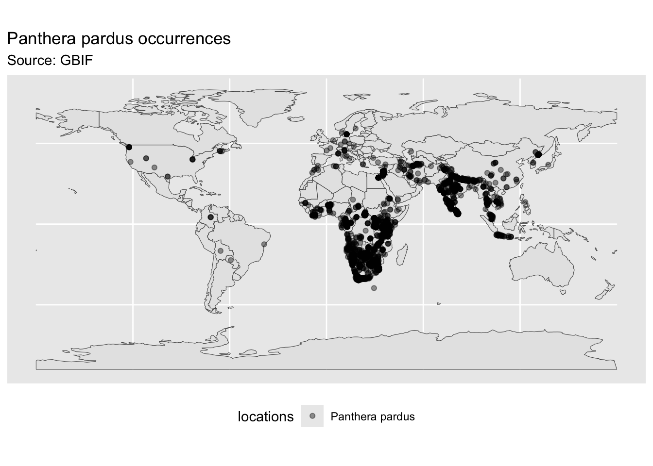
Code
# tmap
tm_shape(pardus_sf) +
  tm_dots(fill = "black", fill_alpha = 0.4) +
  tm_graticules() +
  tm_basemap("OpenTopoMap")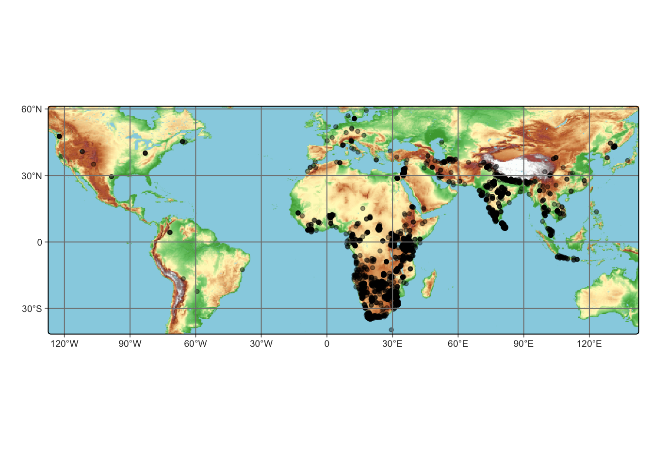
Some thoughts on the initial global map include records indicating leopards occurring in North and South America and Europe, which come as a surprise to me. These were probably occurrences in zoos or other captive facilities listed by public citizens. Thus, it is probably best to know a few things on current distribution of your focal species of interest before integrating records from public databases, such as GBIF. Also, I am aware I did not include a north arrow or scale bar for this map, as this is only a draft and not finalized for any publications.
However, we can create a second map that focuses on Africa and Asia continents to get a clearer look at more natural leopard occurrences. We do this by filtering the areas of interest (Africa and Asia) in our World object. We then make sure the projections for both pardus_sf_aa and africa_asia objects are the same so that we can use the st_intersection() function to clip the locations that fall outside our Africa and Asia polygon, so that points in North America, South America and Europe don’t show up on the map. The st_crs() argument is handy for extracting the CRS information from an object, and the st_transform() argument lets you change the CRS information for a given object. Changing the alpha value on the pardus_sf_aa points can show the density of locations; darker points show us that an aggregation of occurrences are mainly in southern Africa and India.
Code
Coordinate Reference System:
  User input: EPSG:4326
  wkt:
GEOGCRS["WGS 84",
    ENSEMBLE["World Geodetic System 1984 ensemble",
        MEMBER["World Geodetic System 1984 (Transit)"],
        MEMBER["World Geodetic System 1984 (G730)"],
        MEMBER["World Geodetic System 1984 (G873)"],
        MEMBER["World Geodetic System 1984 (G1150)"],
        MEMBER["World Geodetic System 1984 (G1674)"],
        MEMBER["World Geodetic System 1984 (G1762)"],
        MEMBER["World Geodetic System 1984 (G2139)"],
        MEMBER["World Geodetic System 1984 (G2296)"],
        ELLIPSOID["WGS 84",6378137,298.257223563,
            LENGTHUNIT["metre",1]],
        ENSEMBLEACCURACY[2.0]],
    PRIMEM["Greenwich",0,
        ANGLEUNIT["degree",0.0174532925199433]],
    CS[ellipsoidal,2],
        AXIS["geodetic latitude (Lat)",north,
            ORDER[1],
            ANGLEUNIT["degree",0.0174532925199433]],
        AXIS["geodetic longitude (Lon)",east,
            ORDER[2],
            ANGLEUNIT["degree",0.0174532925199433]],
    USAGE[
        SCOPE["Horizontal component of 3D system."],
        AREA["World."],
        BBOX[-90,-180,90,180]],
    ID["EPSG",4326]]
Code
st_crs(pardus_sf)Coordinate Reference System:
User input: EPSG:4326
wkt:
GEOGCRS["WGS 84",
ENSEMBLE["World Geodetic System 1984 ensemble",
MEMBER["World Geodetic System 1984 (Transit)"],
MEMBER["World Geodetic System 1984 (G730)"],
MEMBER["World Geodetic System 1984 (G873)"],
MEMBER["World Geodetic System 1984 (G1150)"],
MEMBER["World Geodetic System 1984 (G1674)"],
MEMBER["World Geodetic System 1984 (G1762)"],
MEMBER["World Geodetic System 1984 (G2139)"],
MEMBER["World Geodetic System 1984 (G2296)"],
ELLIPSOID["WGS 84",6378137,298.257223563,
LENGTHUNIT["metre",1]],
ENSEMBLEACCURACY[2.0]],
PRIMEM["Greenwich",0,
ANGLEUNIT["degree",0.0174532925199433]],
CS[ellipsoidal,2],
AXIS["geodetic latitude (Lat)",north,
ORDER[1],
ANGLEUNIT["degree",0.0174532925199433]],
AXIS["geodetic longitude (Lon)",east,
ORDER[2],
ANGLEUNIT["degree",0.0174532925199433]],
USAGE[
SCOPE["Horizontal component of 3D system."],
AREA["World."],
BBOX[-90,-180,90,180]],
ID["EPSG",4326]]Code
# now union
pardus_sf_aa <- st_intersection(pardus_sf, africa_asia)
# combine sf objects to produce ggplot map
ggplot() +
  geom_sf(data = africa_asia) +
  geom_sf(data = pardus_sf_aa, aes(color = "Panthera pardus"), alpha = 0.4) +
  labs(title = "Panthera pardus occurrences in Africa and Asia",
       subtitle = "Source: GBIF") +
  scale_color_manual(name = "locations",
                     values = "darkorange") +
  theme(legend.position = "bottom")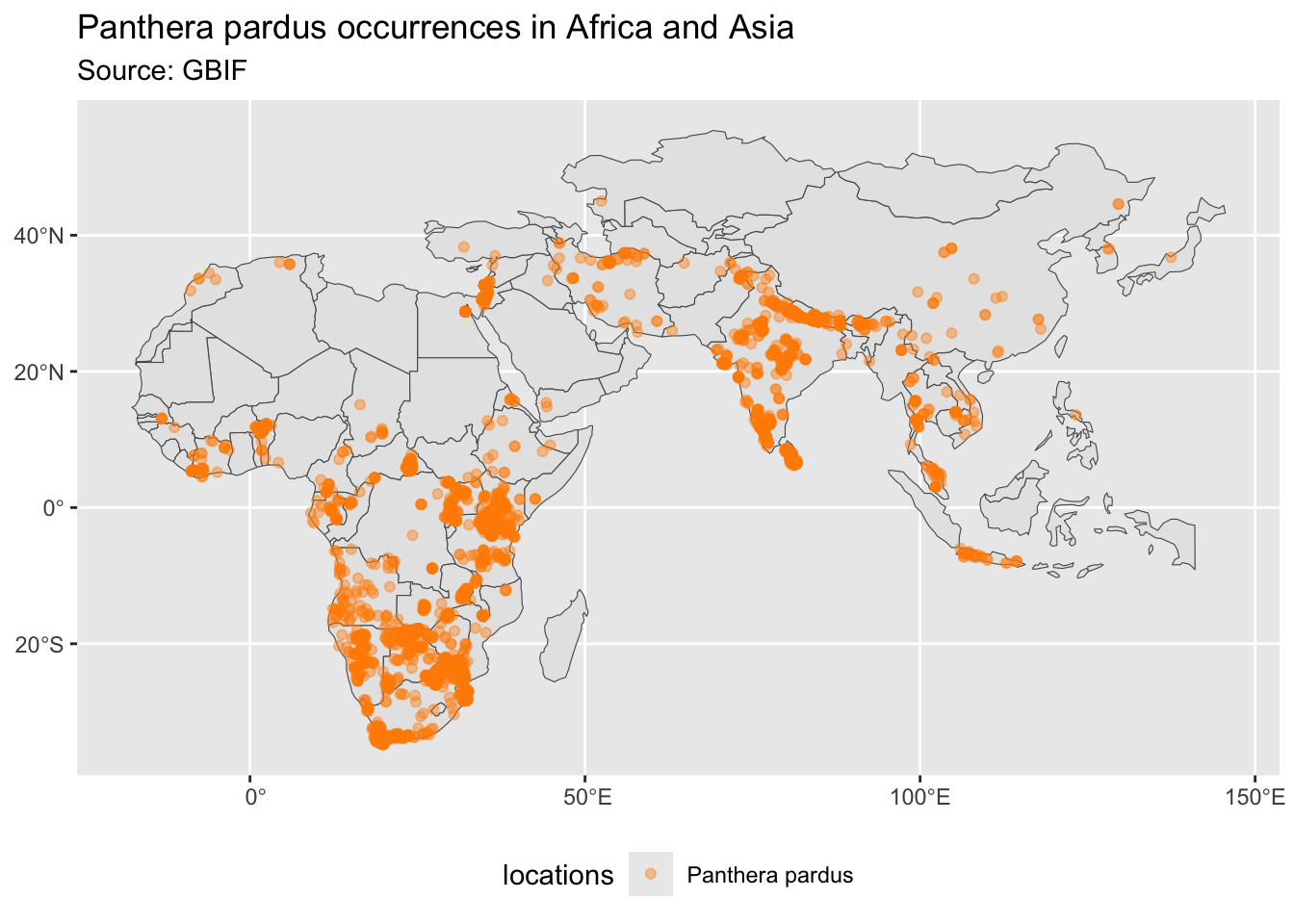
Code
# tmap
tm_shape(pardus_sf_aa) +
  tm_dots(fill = "darkorange", fill_alpha = 0.4) +
  tm_graticules() +
  tm_basemap("Esri.WorldTopoMap")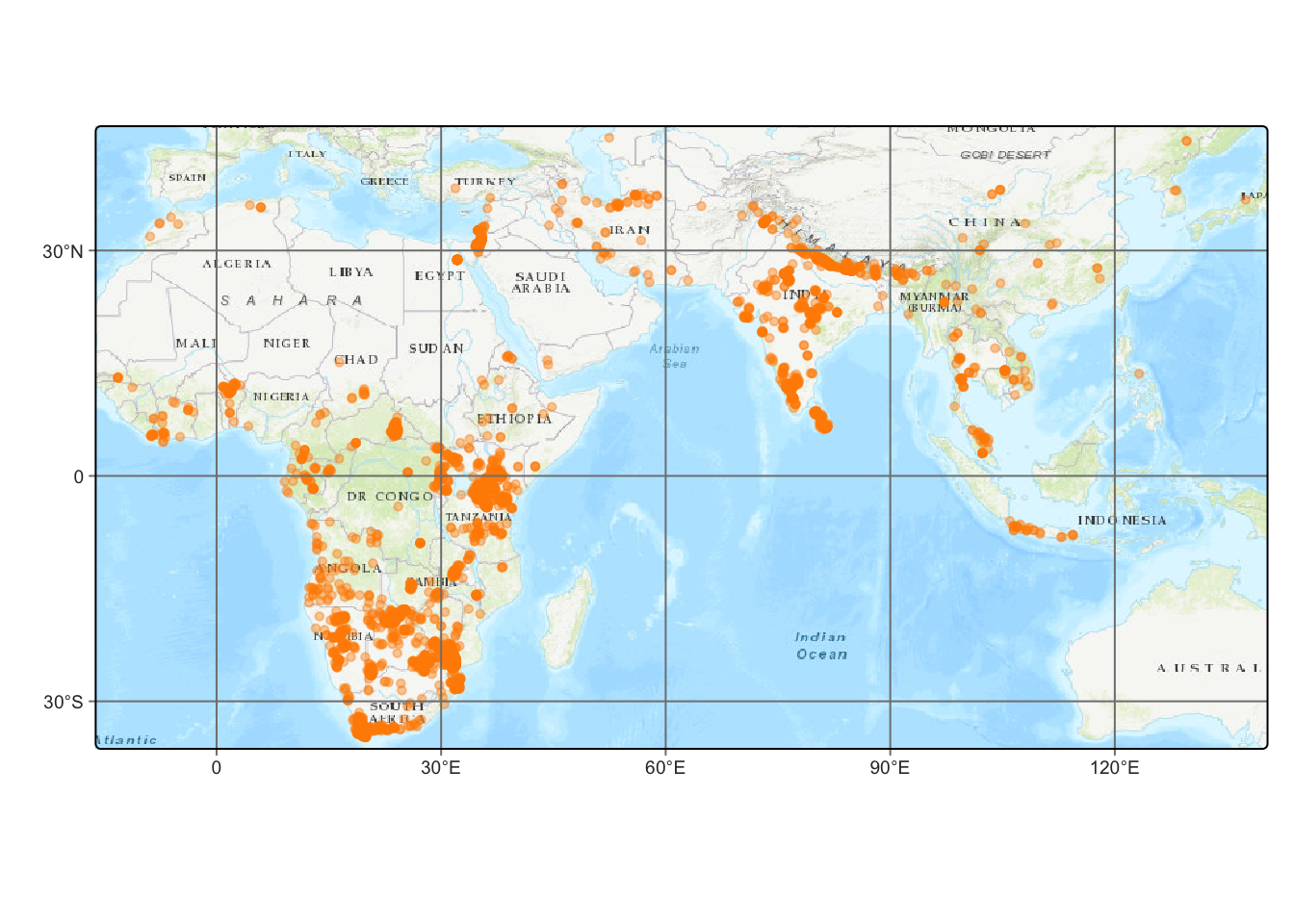
5 Interactive Map
I am also a big fan of producing interactive maps for quicker access to explore the data interactively. tmap provides an html interactive map mode for this task. You’ll notice that the way to produce a tmap is similar to producing a map with the ggplot syntax.
View the interactive tmap!
Code
tmap_leaflet(pardus_int, show = TRUE)